Revisiting AEVB
I went back to reading about TrueSkill, with some vague ideas about adding things like home-advantage, injuries, etc. In the past, I have tried to derive EP updates manually. Even for relatively “trivial” problems it just takes too long. Instead, I started searching for black-box inference techniques. I remembered having played around with PyMC3, and that is supported a framework called ADVI. And that’s where I started – with the ADVI paper. As I worked my way down the rabbit hole of references, I came across AEVB.
Consider the factor graph for TrueSkill.
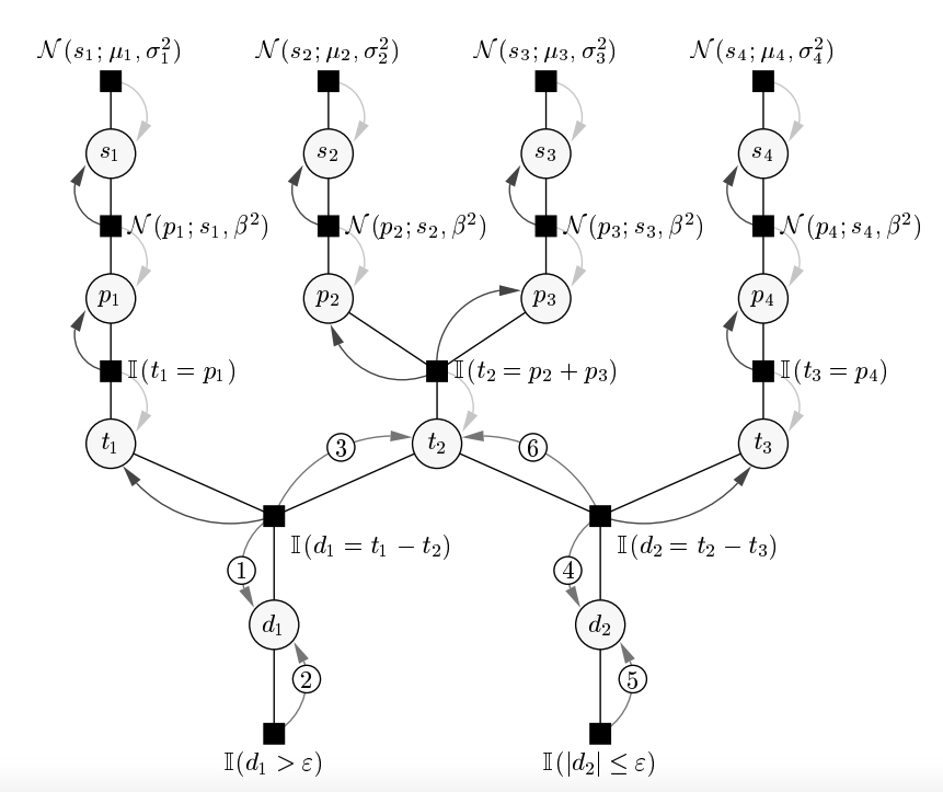
A factor graph of the TrueSkill model for interactions between three teams (1 v 2 v 1).
The goal is to estimate the lantet variables (i.e. skills $\mu, \sigma$), given the observed data (i.e. win/loss events). Note that we only have access to the observed data $x$ – all variables in this graph ($s_i, p_i, d_i, t_i$) are latent variables $z$ introduced by the user. We want an estimate over the probability distribution
\[p(z \mid x) = \frac{p(x \mid z) p(z)}{p(x)}\]For many model descriptions (particularly complex ones) this is intractable.
- For the TrueSkill factor graph, the likelihood is a truncated distribution, along with additions and subtractions of gaussians.
- The denominator would require an integrals over all latent variables.
Variational Bayesian Methods offer a solution:
- Devise an approximate model $q_\phi(z \mid x)$ (aka recognition model) that is well known and tractable.
- Find parameters $\phi$ which minimizes $\text{KL}(q \mid\mid p)$.
- In many cases, you cannot minimize the KL directly, and so you optimize for a different formulation.
This procedure is NOT straightforward.
- You have to make very conscious choices about the form of $q$ so that it remains tractable.
- Even then, all updates have to be derived manually.
- Update derivations for relatively trivial problems are fairly involved. In the Clutter Problem from Minka’s thesis on page 21, the condensed update equations for a single latent parameter span a page and half!
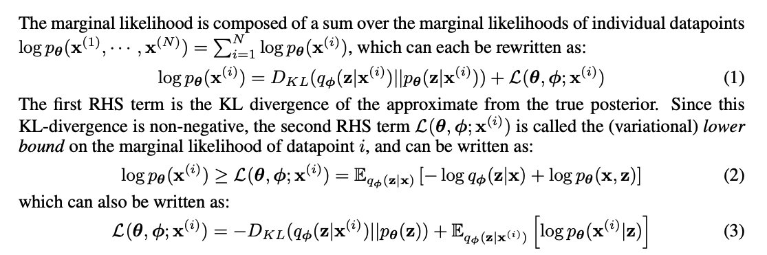
It turns out, that minimizing the KL is equivalent to maximizing the evidence lower-bound (ELBO) – you can show that log-likelihood of the data equals to ELBO + KL (Understanding the Variatioal Lower-Bound).
\[L = \text{log }p(X) - \text{KL}[q(z) \mid \mid p(Z \mid X)]\]The ELBO can be defined as
\[\begin{align} & L = \text{E}_q[\text{log }p(X, Z)] + H[Z] \\ & H[Z] = - \text{E}_q[\text{log }q(Z)] \end{align}\]So, we have established that minimizing the KL-divergence is equivalent to maximizing the ELBO. And we also have a formulation of the ELBO. What if we treat this as the objective, and use SGD to find the latent parameters? This is explored in the AEVB paper.
AEVB
You have a dataset $X$ consisting of $N$ i.i.d. samples. Each point $x^i$ can be continuous or discrete. Data is generated in a 2 step process:
- A value $z^i$ is sampled from the latent variable $z$ with prior probability $p(z)$.
- A value $x^i$ is generated according to conditional probability distribution $p(x \mid z)$.
$z$ is unseen and all parameters in its densities are unknown; if $p(x \mid z)$ is a neural network, then its weights are the parameters $\theta$. We want to estimate the parameters, and the latent variables.
A major contribution of AEVB, is that it makes NO simplifying assumptions about the posterior $p(z \mid x)$, or the marginal $p(x)$. Rather, the authors are interested in generic framework that is applicable in the following scenarios:
- Intractability: Models were the marginal $p(x)$ is intractable, the posterior is intractable, and any integrals required for mean-field approaches are also intractable. In mean-field VI, you introduce an approximation of the true posterior $q_{\phi}(z \mid x)$, and ensure that $q_{\phi}$ can be factorized into some well-known distributions which are tractable. AEVB assumes this form is also intractable.
- Large datasest: Applications where full batch optimization and large-scale sampling methods are not possible. In such cases, mini-batche approach is better suited.
Why call it “Encoder-Decoder”?
From coding theory perspective, $z$ can be interpreted as a latent representation, or a code. Hence, the approximation $q(z \mid x)$ can be thought of as an encoder – given datapoint $x$, the encoder generates a distribution over values of $z$ from which the datapoint $x$ could have been generated.
Similarly, we refer to $p(x \mid z)$ as a decoder that generates a distribution over $x$.
In effect, we are trying to estimate the parameters and the latent variables by:
- Estimating the (distribution over) the lantent variables.
- Sampling from the latent distribution.
- Reconstructing the sample using the likelihood $p(x \mid z)$
The ELBO
We want to find $q_\phi$ that is closest to $p_{\theta}(z \mid x)$. KL divergence gives is one measure. But minimizing it directly is not possible.
ELBO reformulation.
We only care about Eq.3. Expectation is w.r.t $q_\phi$: $\sum_{z} q_\phi (z \mid x)\ \text{log}\ p_\theta(x \mid z)$.
How to interpret this formulation?
The 2nd term is log-likelihood of the given input, for the $z$ that we have sampled. This term will be maximized only when the highest probability is assigned to the original/true value of $x$. Think of this as the reconstruction error.
The first term (KL divergence) is a form of a regularizer. Think back to the normal non-probabilistic auto-encoder.
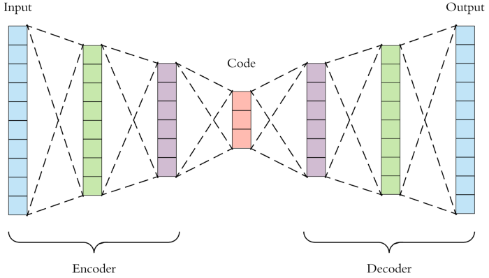
A standard autoencoder.
There is a chance that the network learns to copy the input in the code.
- Limit the number of units – forced to learn only the most representative features.
- Corrupt the input, but use the original in the reconstruction – downsample, noise, etc.
This term forces the encoding to be similar to the prior distribution – if your prior $p(z)$ is a Normal, then this will force the codes to resemble Normals.
There are also some other advantages of sampling:
- It automatically acts as a noise inducer – because you expect similar outputs from nearby samples of a code.
- This is what also ensure a smooth interpolation between two points in the codes space.
SGVB estimator
We want to take derivatives of the ELBO w.r.t $\theta, \phi$ and then optimise using SGD, Adam etc. One issue is that $z$ is still a random variable : $z \sim q_\phi(z \mid x)$. The paper proposes tranform to a differentiable function:
Transform.
This leads to the following approximation of the ELBO:
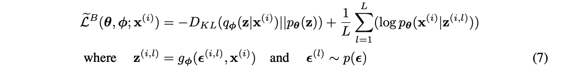
ELBO with sampling.
which can be used with mini-batches, and a single sample L=1.
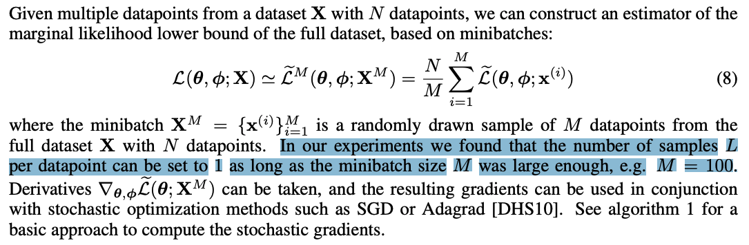
Minibatch estimator.
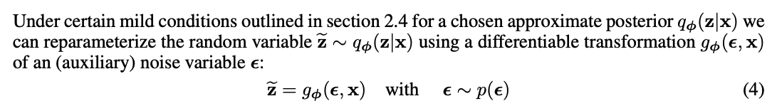
Re-parameterization Trick
In some conditions, it is possible to express random variable z as a deterministic variable z = g(e, x), where $g$ is parameterized by phi.
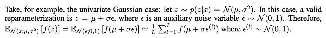
The Normal auxiliary varriable for the AEVB Reparameterization Trick.
AEVB Algorithm
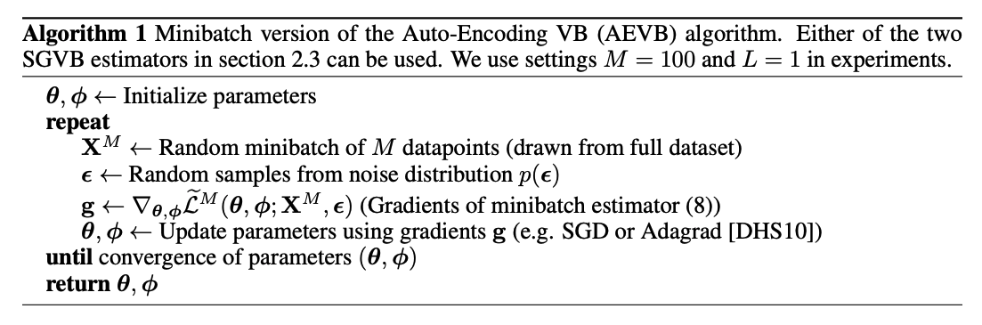
AEVB algo.
And that’s it!
The Re-Parameterization trick was the last piece of the puzzle. To train a Variational Auto-Encoder for generating MNIST digits:
- Feed the Encoder model the input image; this will generate the latent codes.
- If you have $k$ Gaussian codes, you will generate two vectors of size $k$: one for the means, and the other for the sigmas.
- Using the re-parameterization trick, we sample from our auxiliary random variable, scale the sigmas and add to the means.
- We feed this to the decoder, which tries to reconstruct the original image.
- The loss function accounts for both terms (reconstruciton, and prior regularization).
I’ll try to implement a version of this over the next few weeks. Meanwhile, here’s a list of some things I did not discuss…
- Other ELBO estimators, and their tradeoffs. There is a estimator that does not include KL divergence. Another one does not use the Reparameterization Trick, and has higher variance.
- Suggestions on the deterministic differentiable transform function – you can use more than just Gaussians as priors.
- Form of the encoder has a diagonal covariance – assumes all “codes” are independent. This might make some sense for simplistic datasets like imagenet: code0 represents number, code1 represents size, code2 represents thickness, code3 represents tilt, etc … But might not make sense for others. This also simplifies computation – encoder output is just 2xK, where K is dim size of z – first K values are the means, and next K are the std deviations.
- This only works for continuous latent variables – as with SGD. Paper mentions 1 other paper that has comparable time-complexity and is also applicable for discrete vars.